
A robot can receive several depth streams without those streams describing the same instant or sharing a coordinate frame. Combining them immediately may create doubled walls, displaced edges and obstacles that appear to move with the robot. This explainer is for teams building surround-depth perception from rigidly mounted cameras. You will learn how to budget timing error, establish camera-to-body transforms, handle active illumination and estimate data throughput before choosing hardware.
Separate exposure timing, clock alignment and calibration
Multi-camera point cloud synchronization has three independent requirements. First, the cameras must observe the scene at sufficiently similar times. Second, their timestamps must be comparable. Third, their measurements must be transformed into the same coordinate frame.
| Requirement | What it establishes | What it does not establish |
|---|---|---|
| Exposure synchronization | A controlled relationship between acquisition events | Shared coordinates or identical exposure midpoints |
| Clock alignment | Comparable capture timestamps across devices | Simultaneous acquisition |
| Extrinsic calibration | The position and orientation of each camera relative to a reference frame | Timing accuracy or motion compensation |
| Frame association | Which captured frames belong to one fusion group | Correct timestamps or correct calibration |
A shared electrical trigger can coordinate acquisition, but its actual effect depends on the documented camera behavior. Different exposure durations or internal delays can still produce different observation times. Some depth technologies also build a measurement from multiple acquisitions rather than one instantaneous exposure.
Conversely, synchronized clocks can support accurate timestamps while cameras continue capturing at different phases. Software can identify those differences, but cannot turn sequential observations into simultaneous ones.
Do not confuse receiving complete streams with validating their timing. If a depth component is absent or decoded incorrectly, resolve that first using depth-stream and pixel-format troubleshooting. Geometry checks are not meaningful until the underlying measurements are valid.
Set a motion-error budget before choosing synchronization
The allowable time difference depends on robot speed, rotation, scene distance and acceptable registration error. For a stationary scene and small motion, a conservative first-order estimate is:
This bound adds translation and rotational contributions. Their actual vector effects can partially cancel, but designing around cancellation is unreliable. Independently moving objects introduce additional relative motion.
Consider an illustrative rig translating at 0.8 m/s and rotating at 0.6 rad/s. A wall point lies 2 m from the rotation center. The estimated worst-direction relative speed is:
The 3 mm allowance is an example, not a universal requirement. Allocate separate allowances for depth uncertainty, calibration, mounting movement and pose estimation. Timing cannot consume the entire registration budget.
Exposure duration also matters. Even perfectly aligned exposure midpoints cannot eliminate motion during a long acquisition. For depth systems using several patterns or sub-exposures, check the complete measurement interval rather than only the reported exposure setting.
Establish a measurable capture timeline
Start with the manufacturer's documented acquisition and synchronization modes. Confirm whether an input starts an exposure, starts a depth sequence, resets a clock or serves another function. These behaviors are not interchangeable.
For hardware synchronization, verify electrical levels, polarity, pulse width, grounding, connector pinout and permitted loading. Do not connect camera outputs together unless the documented wiring explicitly permits it. Several inputs may require a suitable distribution device rather than an improvised parallel connection.
Separate capture timestamps from host-arrival timestamps. Arrival time includes transport, driver scheduling and queue delays. It can help diagnose latency, but usually provides a poor estimate of when the scene was observed.
If timestamps represent exposure start, equal exposure durations may permit a common midpoint estimate:
Use that conversion only when it matches the documented acquisition model. A depth sequence or rolling acquisition may not have one representative time for every point. See how to verify per-frame exposure metadata when exposure information forms part of your timing calculation.
Where cameras support a common clock mechanism, confirm that it is active and stable. Otherwise, characterize clock offset and drift using a supported method. A one-time offset correction does not establish long-term agreement between free-running clocks.
The fusion software should then:
- Compare capture times expressed in a common clock domain.
- Accept a group only when its latest timestamp minus its earliest timestamp meets the allowed spread.
- Reject stale, missing or unmatched frames instead of silently reusing them.
- Record frame identifiers, capture times, arrival times and rejection reasons.
- Bound queue depth so delayed data cannot masquerade as a current observation.
The distinction between trigger rate and accepted acquisition rate is covered in hardware-trigger frame-rate checks. Apply those checks before blaming the registration algorithm.
Transform every cloud into a defined reference frame
A depth image must first be converted into camera-coordinate points using the correct intrinsics and depth interpretation. Optical-axis depth and radial range require different unprojection equations. Prefer the documented conversion supplied for the measurement format rather than assuming every depth value means the same thing.
Check whether the cloud belongs to the native depth frame or a registered image frame. Resolution changes, cropping and image registration can change which intrinsics and coordinate definitions apply.
For a rigid camera rig, define a body frame and calibrate a fixed transform for every camera:
For observations captured at different times, robot motion must also be considered. With a suitably timestamped body pose, map each observation into a fixed world frame:
To express those observations in the body frame at a chosen reference time:
This compensates for estimated rig motion between captures. It does not correct an independently moving obstacle, inaccurate pose estimates or motion distortion within a depth acquisition.
Calibrate with rigid, well-observed geometry across several positions and orientations. Validate on different geometry afterward; a low fitting error on the calibration data alone is insufficient. The calibration-target flatness guide explains why target shape can limit the result.
Rotation accuracy becomes especially significant at longer distances. An illustrative angular calibration error of 0.2 degrees is approximately 0.00349 rad. At 2 m, its lateral contribution is approximately 2 × 0.00349 = 0.007 m, or 7 mm.
Design overlap without assuming full surround coverage
Adding camera viewing angles does not prove complete coverage. Camera housings, the robot body, payloads, minimum usable range and depth-invalid regions can leave gaps. Check coverage at the heights and distances where obstacles actually matter.
Overlap provides shared surfaces for calibration and independent validation. However, there is no universal overlap percentage that guarantees reliable alignment. A narrow view of a flat wall may constrain some motion directions poorly. Repeated shelving or similar surfaces can also produce plausible but incorrect matches.
Evaluate 3D sensors through the camera finder against usable depth coverage, not only image width. The wide-baseline stereo selection guide provides related guidance on depth geometry; surround-camera fusion adds inter-camera timing and extrinsic requirements.
Active illumination introduces another constraint. Simultaneous emitters can affect depth validity or uncertainty when their illumination reaches the same surfaces. The effect depends on the sensing method, ambient light, materials and documented interference handling.
| Capture approach | Main benefit | Main limitation |
|---|---|---|
| Simultaneous acquisition | Small inter-camera capture-time spread | Active emitters may interfere |
| Time-multiplexed acquisition | Separates illumination intervals | Creates sequential observations and reduces timing margin |
| Documented interference-management mode | May support coordinated active operation | Availability and performance must be verified for the selected devices |
For illustration, four sequential acquisition slots lasting 5 ms each require at least 20 ms per cycle before overhead. The first and last slot midpoints are 15 ms apart. Translation at 0.8 m/s alone produces 0.8 × 0.015 = 0.012 m, or 12 mm, of displacement.
This is why time multiplexing is not a free replacement for synchronization. Validate it at maximum operating motion, and include the camera's full illumination sequence when defining each slot.
Budget transport and cloud-processing bandwidth separately
Estimate the depth-image payload before adding color, confidence data or generated point clouds. For uncompressed depth data:
An illustrative four-camera system using 640 × 480 depth images, 2 bytes per pixel and 30 frames/s produces:
These are decimal megabytes. The estimate excludes protocol overhead, metadata, retransmission and additional image components. Nominal interface speed is not the same as sustained application throughput.
Generating an XYZ cloud with three 32-bit floating-point coordinates requires 12 bytes per point before padding or other fields:
That is six times the raw depth payload. Memory copies, coordinate transforms and serialization add processing work even when the camera links are operating normally.
Check shared interface controllers and uplinks, not just connector count. Compare vision controllers against measured acquisition and processing loads; a port count does not establish independent bandwidth or synchronization support.
Use bounded queues and monitor processing age. A 250 ms backlog at 0.8 m/s represents 0.20 m of robot travel. If callbacks stall or queues grow, use the multi-camera acquisition-freeze troubleshooting guide to separate transport problems from application scheduling.
Treat catalog parts as candidates, not a validated synchronized kit
The MV-DPS200P-02 is cataloged as a projected structured-light 3D camera. Consider it as a sensing-method candidate, with synchronization behavior and interference handling still requiring documentation review.
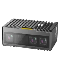
- Type
- Stereo / structured light
The MV-DT01WMU is cataloged as a ToF sensing camera. That classification alone does not establish its timestamp semantics, trigger capabilities or suitability for a mobile rig.
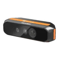
- Type
- Depth / ToF camera
These listings do not establish mutual compatibility or provide a recommended mixed-camera arrangement. Before ordering, request the timing definitions, acquisition sequence, software interface, calibration access and operating limits needed by your design.
Specify cables from verified connector and electrical requirements. Use the accessory finder and cable configuration step after confirming pinouts, routing, strain relief and movement requirements.
Camera data, power and I/O cables
366 models · from $39.00Verify the system in stages, and recognize its limits
Validate stationary geometry first, then add motion and computational load. This order helps distinguish calibration faults from timing faults and processing delays.
- Stationary overlap: compare independent views of the same surfaces without robot motion. Persistent offsets suggest geometry, depth bias or calibration problems.
- Translation test: repeat the observation at increasing speed. Error that grows with speed points toward timing or pose alignment.
- Rotation test: observe features at several distances. Error growing with distance can expose angular calibration or timing problems.
- Emitter test: compare each camera operating alone with all cameras active. Track invalid-depth fraction and surface scatter, not just visual appearance.
- Load test: record timestamp spread, dropped frames, queue age and processing duration under the intended operating load.
- Restart test: verify clock alignment, frame association and calibration selection after power cycles and reconnects.
- Coverage test: inspect the actual robot envelope, including near-body gaps, payload occlusion and difficult surfaces.
Do not accept a fused cloud merely because smoothing makes it look continuous. Averaging can hide doubled surfaces while preserving an incorrect obstacle position. Keep individual camera contributions available during commissioning.
Motion compensation is not a substitute for simultaneous capture when moving objects dominate the task. Likewise, low average timestamp error does not excuse occasional large mismatches; acceptance limits should cover the intended operating envelope.
Document the allowable timing spread, calibration residuals, processing age and coverage gaps as separate acceptance criteria. Take those requirements to the camera configuration step, or contact the applications team with your motion envelope, working distances and proposed capture schedule before selecting parts.
Questions
Do all depth cameras need a shared hardware trigger?
Not necessarily. Hardware triggering is useful when the application needs tightly coordinated observations, but some systems can associate independently captured frames using comparable timestamps and motion estimates. The decision depends on the allowable geometric error, robot motion and scene motion. Confirm the actual capture-time spread rather than assuming a particular synchronization method is sufficient.
Can calibration remove the effects of capture-time differences?
No. Coordinate transforms place measurements into a shared frame, but observations of a moving object still represent different object positions. Robot-pose compensation corrects the estimated motion of the camera rig, not independent scene motion. Reducing the acquisition-time difference remains valuable even with accurate calibration.
Why does depth quality change when every camera is running?
Active illumination can interact across cameras, reducing valid depth or increasing measurement scatter. Shared transport resources and processing overload can produce different symptoms at the same time. Compare isolated-camera measurements against simultaneous operation while logging depth validity, frame delivery and processing age to distinguish these causes.
Should the application transport depth images or XYZ clouds?
Neither representation is universally better. Raw depth is usually more compact, while XYZ points may simplify downstream geometry. Compare transport payload, conversion cost, memory copies and the fields your application actually needs. Avoid publishing dense clouds repeatedly when the consumer only needs a filtered subset or occupancy representation.
What should be confirmed before buying cameras for a synchronized rig?
Request documentation for trigger behavior, timestamp meaning, clock alignment, depth acquisition duration, emitter coordination and software access to calibration. Also verify electrical connections and sustained interface throughput. Product type and connector count alone cannot establish that several cameras will form a suitable synchronized rig.