
A detector can identify which object to approach without providing enough geometry to orient the tool. This distinction matters when you must visit several objects and approach each surface perpendicularly. A bounding-box center and a depth reading describe a point, not the surrounding surface. You need additional measurements to distinguish centering, distance and tilt errors. The practical task is to select features that constrain those motions, while preserving target identity and rejecting unreliable geometry.
Match each measurement to a commanded motion
Start by defining what perpendicular means: the tool approach axis should align with the local surface normal. This does not necessarily mean pointing toward the camera's optical center or the object's geometric center.
The measurements below provide different geometric constraints. Their actual usefulness also depends on calibration, visibility and the rank of the control Jacobian.
| Measurement | What it constrains | What remains unresolved |
|---|---|---|
| Image center | Two image-coordinate errors | Distance and independent orientation |
| Image center plus valid depth | Position of a visible point | Surface orientation |
| Surface normal | Two orientation components | Rotation around the normal |
| Point plus surface normal | Position and approach-axis alignment | Rotation around the normal |
| Point, normal and an in-plane direction | A complete local target frame | Ambiguities from symmetry or unreliable features |
A point expressed through image coordinates and depth supplies three scalar measurements. It cannot uniquely constrain six independent rigid-body motions. Translation and rotation can produce similar changes in those measurements.
Adding a normal usually supplies the missing tilt information. However, the resulting task still leaves rotation around that normal free. That is acceptable for an axisymmetric tool, but not for a keyed insertion or an oriented gripper.
This measurement question comes before gain tuning or controller selection. The related visual servoing loop design guide covers loop behavior; here, the priority is whether the selected features actually describe the intended motion.
Build a target point from registered depth
A bounding box often includes background, adjacent parts or empty space between object features. Even its center can fall outside the visible object. A segmentation mask is a better starting region, but it is not proof that every enclosed depth sample belongs to the intended surface.
Use a mask associated with the selected target, then exclude invalid depth, boundaries and obvious discontinuities. Confirm that the depth and image coordinates are registered using the correct calibration. Resizing or cropping an image changes the pixel-coordinate mapping unless the transformation is accounted for.
For a calibrated perspective camera, unprojection is:
Here, focal lengths and pixel coordinates use pixels, while Z and the resulting point use the same distance unit. This expression requires axial depth along the optical axis. A sensor reporting radial range needs the appropriate conversion before using this formula.
If the chosen image center has no valid depth, do not silently substitute the nearest available reading. Instead, define an explicit alternative: a visible surface centroid, a fitted-plane intersection, or a rejected observation. Those choices represent different physical targets.
Compare 3D sensors by their suitability for the actual surface and working volume. The camera finder provides a starting point for comparing sensor types, not evidence that every model supplies interchangeable depth data.
The MV-DPS200P-02 is a projected structured-light camera. The MV-DT01WMU is a ToF sensing camera. Confirm depth access, calibration data and application suitability before selecting either:
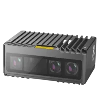
- Type
- Stereo / structured light
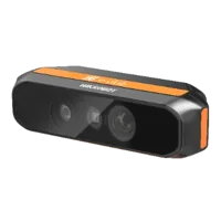
- Type
- Depth / ToF camera
Estimate a surface normal and its confidence
Collect valid points from a patch around the intended contact or approach location. Fitting the whole segmented object can produce a misleading normal when the object has multiple faces or substantial curvature.
For an approximately planar patch, estimate a centroid and fit a plane through the surrounding points. A common least-squares method forms their covariance matrix and selects the eigenvector associated with its smallest eigenvalue as the normal.
Outliers can distort this result, so use an appropriate robust fitting method or reject inconsistent samples before refitting. Assess residuals, spatial coverage and normal stability across successive observations.
Point count alone is insufficient. For example, 100 samples spread across a broad patch can constrain tilt better than 1,000 samples clustered along a narrow strip. Nearly collinear samples leave one tilt direction poorly determined.
A plane normal also has a sign ambiguity: n and −n describe the same plane. Apply a consistent convention, such as choosing the visible normal toward the camera, and check that the resulting approach direction is physically appropriate.
Check alignment using a suitable target before blaming the fit. The calibration target flatness guide explains why reference geometry matters. If depth is absent or misinterpreted, diagnose the depth-stream pixel format before attempting surface estimation.
Choose image-based or position-based errors
Image-based visual servoing controls errors in image-derived features. Position-based visual servoing controls errors in reconstructed spatial geometry. Both approaches require measurements that observe the commanded motion.
Image-based feature combinations
You can combine different feature types by stacking their errors and their corresponding interaction-matrix rows. Each row must describe how its own feature changes under the same camera velocity convention.
For a locally planar target near a front-facing orientation, an illustrative feature vector is:
The normal components are camera-frame quantities. Using n_x and n_y as orientation coordinates is a local choice, requiring a consistent normal sign and a nonzero n_z. It is not a globally valid orientation representation.
Do not append normal errors to a point-feature controller while retaining only the point-feature interaction matrix. The added rows must model the normal's actual motion. Otherwise, the numerical solve treats unrelated quantities as though they had the same geometry.
A five-feature task should not be expected to specify a unique six-axis motion. Use task constraints, secondary objectives or an additional independent feature as appropriate. Check matrix rank and conditioning throughout the expected operating region.
Position-based geometric errors
When reliable depth is available, position-based control can make the perpendicular-approach requirement easier to express. Define a target point, an outward normal and a desired stand-off distance in one common frame.
The tool reference point must be the calibrated point relevant to the task. Camera position is not a substitute for tool position.
Approach-axis alignment supplies two independent orientation constraints. A local cross-product error can represent this alignment, but it also becomes zero at opposite alignment. Resolve direction explicitly and reject configurations outside the controller's intended convergence region.
A full orientation error requires a complete target frame, including an in-plane direction. A fitted normal alone does not provide that frame.
Work through a centering and tilt example
Consider an illustrative calibrated image with focal lengths of 800 px and principal point at (640, 480) px. The selected target point is at (680, 456) px, with axial depth of 0.600 m.
The point is therefore approximately 30 mm horizontally and −18 mm vertically from the optical axis at that depth. These are camera-frame point coordinates, not robot translation commands. A change in camera orientation also changes the point's image position.
Now suppose the fitted unit normal toward the camera is approximately (0.100, 0, −0.995). Its tilt from the backward optical axis is:
Another surface could have exactly the same center pixel and center depth, yet have zero tilt. That is why center and depth cannot determine perpendicularity.
For an illustrative stand-off of 0.100 m, the geometric goal becomes:
The stand-off follows the normal rather than simply subtracting distance from camera Z. Before using this goal, transform it into the controller's required frame and account for the calibrated tool offset.
Keep units, coordinate frames and target identity explicit
Mixed features need meaningful scaling. Pixel errors, distance errors and orientation errors cannot be compared simply because they occupy neighboring vector entries.
One practical approach normalizes errors by acceptable residuals. Illustrative tolerances of 2 px, 2 mm and 1 degree turn those different errors into comparable dimensionless quantities. If a feature row is scaled, scale its corresponding Jacobian row consistently.
Weighting by estimated uncertainty can also help, provided uncertainty is credible. A nearly invalid normal should trigger rejection or a restricted task, not merely receive a small weight while unrestricted motion continues.
Document the frames used for points, normals, velocities and tool offsets. In an eye-in-hand arrangement, the camera-to-tool calibration connects visual measurements to the controlled tool. Transforming a velocity between offset frames requires the appropriate rigid-body velocity transformation, not only rotating its linear component.
The camera integration guide addresses image-input adaptation. Preserve timestamps and calibration metadata through that interface so measurements and robot states refer to compatible acquisition times.
For multiple objects, maintain an explicit target identifier. Detector output order is not an identity guarantee. Associate observations using suitable spatial, appearance and task constraints, and reject ambiguous switches. When the selected target disappears, suspend the approach rather than substituting whichever detection is nearest the image center.
Center, align and approach as separate verified stages
Sequential stages make behavior easier to diagnose, although their geometric errors remain coupled. Tilting an eye-in-hand camera can move the target away from image center, so each stage should keep monitoring the other errors.
- Acquire and identify. Select the intended object and verify sufficient valid depth within its local surface patch.
- Center at a conservative stand-off. Reduce lateral error while checking visibility and tool-clearance constraints.
- Align the approach axis. Use the fitted normal, maintaining position constraints rather than allowing uncontrolled translation.
- Advance along the accepted direction. Continue checking target identity, geometric confidence and remaining stand-off.
- Verify completion before selecting another object. Record the completed target and require an explicit transition to the next one.
Use acceptance bands and dwell conditions instead of advancing after a single favorable frame. For example, a stationary commissioning test might require five consecutive accepted observations. The appropriate count depends on acquisition rate, latency and the application's dynamics.
Ordinary perception and servo software are not substitutes for machine safety functions. Commission within the machine's documented safe operating procedures, with independent protective measures appropriate to the application.
Select hardware without assuming missing capabilities
Choose hardware after defining required measurements. A monocular image can provide detection features, but arbitrary surface orientation generally needs additional geometry, known object structure or other independent information.
For a separate detection channel, compare area scan cameras against image quality, shutter behavior and interface requirements. The LS-MV-133GM-GE is a monochrome, global-shutter GigE camera. Its catalog identification does not imply that it supplies depth or a surface normal.
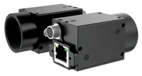
- Sensor format
- 1/2.7"
- Interface
- GigE
- Resolution
- Up to 3 MP
- Shutter
- Global
A separate image and depth channel also introduces registration, synchronization and mounting requirements. The wide-baseline stereo selection guide is relevant when evaluating stereo geometry and depth coverage.
Compare vision controllers against camera connectivity, software compatibility and processing requirements. A controller's available interfaces do not establish compatibility with a particular reconstruction or servoing library.
The usual center-plus-normal approach is wrong when the surface patch is curved, transparent, poorly measured or unrelated to the intended contact geometry. A sphere requires a local contact normal, while a keyed component also requires an in-plane orientation reference. Do not force either task into an unsupported plane model.
Check the measurement contract before ordering
Use this checklist to turn the intended motion into verifiable requirements:
- Target point: Define whether it means mask centroid, visible surface centroid or a designated task location.
- Depth convention: Confirm axial depth versus range, valid-data flags and registration.
- Normal support: Specify the surface patch, minimum spatial coverage and rejection criteria.
- Orientation freedom: Decide whether rotation around the normal is free or explicitly controlled.
- Frames and timing: Record calibration transforms, tool offsets and measurement timestamps.
- Identity: Define target association, loss handling and completion state.
- Verification: Test incorrect masks, missing depth, opposite normal signs and near-degenerate geometry before motion commissioning.
Start a camera configuration once those requirements are clear. If the sensing method remains uncertain, send the surface description, working geometry and required approach accuracy through applications support before choosing parts.
Questions
Are a bounding-box center and depth enough for perpendicular approach?
They can locate a visible point when calibration and depth registration are valid, but they do not establish surface orientation. Perpendicular approach requires a normal or equivalent orientation information. You must also define what the center represents, because a bounding-box center can fall on background or outside the visible surface.
Can image position, depth and surface-normal features be combined?
Yes, provided each feature has a valid interaction model expressed using the same velocity and coordinate conventions. Stack the feature errors and corresponding Jacobian rows, then apply consistent scaling. Combining more features does not automatically remove ambiguity; independence, conditioning and measurement quality still determine which motions are constrained.
Does a fitted surface normal determine the full tool orientation?
A normal specifies an axis direction, leaving rotation around that axis unresolved. That remaining freedom may be acceptable for a rotationally symmetric tool. An oriented gripper or keyed operation needs another independent reference, such as a reliable edge direction, identifiable landmarks or a registered object model.
Should the plane fit use the entire segmentation mask?
Fit a patch that represents the intended approach or contact region. A large patch can improve noise averaging on a genuinely planar face, but spanning multiple faces or curved regions biases the result. Evaluate spatial coverage, fit residuals and stability rather than relying only on the number of points.
How should the system handle several detected objects?
Keep an explicit target identity and associate new observations with that target rather than relying on detection order. Define behavior for occlusion, ambiguous matches and target loss. The approach should suspend when identity becomes uncertain, with a deliberate transition required before selecting another object.