
A coated rod can have the correct outside diameter while its metal core sits off-center. That distinction determines whether an inline inspection station needs cameras alone or a coordinated optical and core-location system. For rods crossing a conveyor at 1,000 parts per minute, measurement access and part tracking matter as much as image resolution. The design below separates the measurements, develops an illustrative timing and uncertainty budget, and identifies what must be demonstrated before ordering hardware.
Define diameter and eccentricity separately
Start with a measurement specification, not a camera resolution. For this example, assume a nominal core diameter of 3 mm and a coated outside diameter of 5 mm. These are application dimensions, not equipment specifications.
For circular, concentric sections, nominal radial coating thickness is:
Eccentricity is the distance between the outside-profile center and the core center at the same axial location. It is not the difference between maximum and minimum outside diameter. A perfectly circular outer surface can conceal an eccentric core.
Define whether you need one section, several positions along the rod, or continuous axial coverage. A measurement near one end does not establish coating thickness throughout the length.
Also clarify what the 0.04 mm requirement means:
- Maximum permissible measurement error against a reference?
- Expanded measurement uncertainty at a stated coverage factor?
- Repeatability under unchanged conditions?
- Total permitted variation in the manufactured part?
These requirements lead to different acceptance tests. Treating them as interchangeable can produce a station that passes repeatability checks but makes incorrect acceptance decisions.
Assign each measurement to a suitable sensing method
A backlit camera measures the outer silhouette. With appropriate optics, calibration and mechanical control, it can measure projected outside diameter and the midpoint between opposing edges.
It cannot directly locate a concealed core through an opaque coating. Adding more pixels or projecting a laser line does not remove that visibility limit.
| Measurement | Suitable approach | Main limitation |
|---|---|---|
| Projected outside diameter | Backlit camera with calibrated optics | One view does not describe every direction around the section |
| Outside-profile center | Opposing silhouette edges in a defined coordinate system | A midpoint is not necessarily a fitted circular center on an irregular section |
| Concealed core position | Qualified electromagnetic or other penetrating measurement method | Response depends on materials, geometry and calibration |
| Core eccentricity | Registered outer-center and core-center measurements | Both measurements must refer to the same section and coordinates |
For a ferrous core, investigate a specialist electromagnetic gauging arrangement capable of estimating core position, rather than merely detecting metal presence. Opposed or multi-direction sensing may be necessary.
A non-ferrous coating is not necessarily electrically insulating. Conductivity, permeability, coating thickness and nearby metal can change sensor response. Require representative sample trials before selecting a core-location method.
Build the optical station around measurement access
The rod must pass between the camera and backlight without the conveyor obscuring the measured edges. An opaque belt beneath the part can prevent the required optical path.
Possible arrangements include a controlled transfer gap, appropriately spaced supports or a carrier with a measurement opening. Support the rod outside the measurement region. Check that the arrangement controls bounce and rotation without deforming the coating.
For the optics, telecentric lenses reduce magnification changes caused by displacement along the viewing direction, within their specified operating limits. They do not eliminate defocus, residual distortion or errors from tilted parts.
The telecentric gauging guide explains that optical decision in more detail. Here, the additional requirement is registering the optical measurement to a separate hidden-core measurement.
The LS-S18WK03X180W is an object-side telecentric, C-mount candidate. Confirm field coverage, sensor coverage, clearance and calibrated performance before treating it as a matched solution.
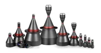
- Sensor format
- 1/1.8"
- Mount
- C-mount
- Image circle
- 8-11 mm
- Type
- Object-side telecentric
Use the lens finder to establish coverage and working-distance options. The optical envelope must also leave room for supports, the core sensor and maintenance access.
For moving parts, start with global-shutter area scan cameras. Monochrome acquisition is appropriate when the measurement depends on silhouette edges rather than color.
The LS-MV-133GM-GE provides a global shutter, monochrome imaging, GigE interface and C-mount. Its suitability still depends on confirming trigger facilities, exposure limits and sustained acquisition performance.
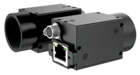
- Sensor format
- 1/2.7"
- Interface
- GigE
- Resolution
- Up to 3 MP
- Shutter
- Global
Compare candidates in the camera finder. Do not infer achievable triggered throughput from resolution or interface type alone.
Choose a backlight by edge behavior
Backlights should produce a stable, high-contrast silhouette across the complete permitted part-position envelope. Avoid saturation and assess the edge transition on actual coated samples.
Collimated illumination can reduce edge-position sensitivity to illumination angles, but its benefit depends on the coating and optical arrangement. Diffuse illumination may be sufficient when the edge remains stable through the allowed height and position range.
The LS-2PFT120120 is a collimated backlight candidate. The LS-LBSS-H-150-150-R2 provides a standard flat-backlight alternative for comparison during sample trials.
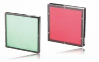
- Size
- 100-200 mm
- Type
- Collimated
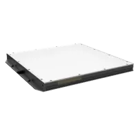
- Size
- 100-200 mm
- Type
- Standard
Use the lighting finder to compare illuminated area and illumination type. Confirm electrical compatibility and permitted operation before choosing a controller or pulse duration. A light category alone does not establish its allowable strobe conditions.
Test whether changing brightness shifts the reported edge. Translucent coatings, scattering, surface fibers and threshold settings can move the apparent boundary even when the physical diameter is unchanged.
Convert conveyor throughput into exposure and tracking requirements
A rate of 1,000 parts per minute gives:
That is the arrival interval, not the allowable exposure time. Motion blur depends on conveyor speed during exposure.
For an illustrative pitch of 30 mm:
This example limits blur to 5 µm in object space. Demonstrating adequate signal at that exposure is a separate lighting test; it is not a performance claim for the candidate hardware.
If each part requires three images, the average acquisition demand becomes approximately 50 images/s. Allow additional capacity for arrival variation, readout and processing queues. Demonstrate sustained operation with the intended image dimensions and camera settings.
Use a part-presence trigger and encoder-based tracking where speed can change. Associate every optical result, core result and reject command with the same part identifier.
For example, a reject point 150 mm downstream corresponds to five pitches in this layout. At the illustrative speed, travel time is 0.30 s. Encoder position is preferable to a fixed delay when acceleration or stopping is possible.
The camera-selection guide for handled parts provides related discussion of presentation and acquisition choices. Conveyor integration adds the need to preserve result identity through every downstream action.
Size image sampling without confusing it with accuracy
Choose the field of view from the maximum outside diameter, lateral movement and required background margins. Then calculate object-space sampling along the measurement direction.
Consider a hypothetical image with 1,000 usable pixels spanning a 10 mm field:
These are illustrative image requirements, not verified operating settings for the listed camera and lens. Actual coverage follows from sensor dimensions and lens magnification.
Subpixel edge fitting can improve repeatability, but it does not establish absolute measurement accuracy. Calibration error, coating appearance, part tilt and temperature remain even when a fitted edge moves by a small fraction of a pixel.
Measure opposing edges at multiple positions along a selected axial window. Report local widths or fitted geometry according to the specification. Avoid averaging away a short, unacceptable coating defect merely to obtain a quieter diameter result.
Register core position to the optical measurement
The core sensor must deliver a position estimate in coordinates that can be related to the outer-profile measurement. A scalar coating-thickness reading at one location is not automatically a complete core-center measurement.
For circular sections, define eccentricity as:
A single silhouette view supplies only one projected center coordinate. Full cross-sectional eccentricity requires sufficient independent directional information from the combined sensing arrangement. Two orthogonal optical projections can help establish the outer center for a circular section, but still do not reveal the hidden core.
Register the sensing stations using suitable reference pieces with independently established outer and core geometry. If measurements occur at separate conveyor positions, confirm that rolling, axial sliding and tilt do not change the correspondence.
For ideal circular sections with known radii:
Using the example diameters and an eccentricity of 0.10 mm gives minimum thickness of 1.00 − 0.10 = 0.90 mm and maximum thickness of 1.00 + 0.10 = 1.10 mm.
These equations do not describe local thickness reliably when either boundary is irregular. Nominal core diameter also cannot substitute for measured core geometry when its variation matters.
Validate uncertainty against the actual acceptance requirement
Build separate uncertainty budgets for outside diameter and eccentricity. Good diameter performance does not establish good core-location performance.
For illustration, suppose a diameter study establishes these standard uncertainty contributions:
| Contribution | Illustrative standard uncertainty |
|---|---|
| Calibration and reference transfer | 0.004 mm |
| Repeated dynamic measurements | 0.005 mm |
| Residual depth and alignment effects | 0.003 mm |
| Temperature-related effects | 0.002 mm |
If these contributions are appropriately evaluated and independent, their root-sum-square combination is:
This is an illustrative expanded uncertainty at coverage factor k = 2, not a prediction for the proposed station. Correlated effects require covariance terms; unknown biases cannot simply be treated as independent noise.
An expanded uncertainty of 0.015 mm is below a requirement explicitly defined as 0.04 mm expanded uncertainty. It may still be inadequate if 0.04 mm is the entire product tolerance width.
For example, a centered tolerance with limits at ±0.020 mm leaves only ±0.005 mm for guarded acceptance if the agreed rule keeps the complete ±0.015 mm uncertainty interval inside those limits. Set the decision rule with the quality team before commissioning.
For eccentricity, include core-sensor error, outer-center error, coordinate registration and section matching. Near zero eccentricity, the magnitude calculation has nonlinear behavior. Evaluate coordinate errors and representative concentric samples rather than relying on percentage repeatability of the reported magnitude.
Prove the complete station under production conditions
First establish reference values using a method with suitable traceability and uncertainty. For core eccentricity, selected cross-sections may require independent sectional examination or another qualified reference method.
Use representative samples spanning acceptable and unacceptable diameter, offset, coating appearance and material variation. Include controlled differences in core size where those occur in production.
Separate several tests:
- Measure stationary references to establish bias and short-term repeatability.
- Repeat measurements across the permitted height, lateral position and tilt envelope.
- Run identified samples dynamically at minimum, nominal and maximum production speeds.
- Test optical-to-core registration after realistic part movement between stations.
- Challenge missed triggers, touching parts, failed core readings and processing timeouts.
- Verify that the reject mechanism acts on the intended part and confirms removal.
Record raw images, sensor outputs, encoder positions and decision reasons during qualification. Compare stopped and moving results to identify errors caused by presentation rather than calibration.
An incomplete measurement must produce a defined disposition, not an automatic pass. Specify whether the line rejects that part, diverts it for reinspection or stops under the machine's validated operating design.
Know when to change the architecture
Use additional viewing directions when out-of-roundness matters. One projected width cannot establish roundness, and two widths may still miss localized lobing.
Consider end-face imaging only when the core is visible and the required measurement genuinely concerns that end. A visible end does not prove the condition of concealed sections farther along the rod.
Structured-light profiling can help measure accessible outer-surface shape or height. It does not locate a concealed core through an opaque coating, and surface reconstruction brings its own calibration and visibility limits.
If coating conductivity or surrounding metal prevents adequate electromagnetic core localization, reconsider the sensing method, shielding layout or inspection location. Do not compensate for an unobservable core position by assigning an optical result a different label.
Before ordering, complete this handoff checklist:
- Define the measurands, axial coverage and meaning of the 0.04 mm target.
- Supply representative samples and independently established reference values.
- Confirm optical access, sensor clearances and non-deforming part support.
- Verify camera triggering, exposure, throughput and image transfer experimentally.
- Establish core-location capability and coordinate registration separately.
- Agree uncertainty limits, acceptance rules and failure dispositions.
- Validate tracking, rejection and safe machine integration as one system.
Start the optical layout with the camera configurator. For the combined measurement design, send the sample dimensions, material information, conveyor layout and acceptance specification through application support so the optical station and core-location requirement can be assessed together.
Questions
Can a camera measure eccentricity through an opaque coating?
A camera can measure the visible outer boundary, but an opaque coating prevents it from directly observing the core. Eccentricity therefore needs an independently validated core-position measurement registered to the optical coordinates. Imaging an exposed end is an alternative only when that end is the required inspection location.
What camera speed is needed for 1,000 rods per minute?
The part arrival rate is approximately 16.7 parts per second, but exposure depends on conveyor velocity and permitted blur. Multiple views or repeated captures increase acquisition demand. Select hardware only after testing sustained triggered operation, illumination, processing capacity and downstream part tracking together.
Does sufficient pixel resolution guarantee the 0.04 mm target?
No. Pixel spacing describes sampling, while accuracy also depends on reference calibration, optics, presentation, edge behavior and environmental effects. First define whether the target means error, repeatability, uncertainty or product tolerance, then demonstrate the corresponding performance using representative reference samples.
Will a magnetic sensor work with any non-ferrous coating?
A material described as non-ferrous may still conduct electricity and influence electromagnetic sensing. Core alloy, magnetic properties, coating composition, temperature and nearby structures can all affect interpretation. Require trials that demonstrate core-position accuracy across the actual material and geometry range.
Is a collimated backlight always necessary?
Not necessarily. A stable diffuse silhouette may satisfy the measurement requirement, while collimated illumination can help when illumination angle affects the apparent edge. Compare both on actual samples through the permitted position range, including brightness changes and the exposure required during motion.